Application to Scheduling Problems (Part 2)

Note

This article explores the application of optimization to scheduling problems. We will explain in detail the formulation introduced in Application to Scheduling Problems (Part 1).

1. Overview: Recap of Part 1

This page provides a step-by-step explanation of the mathematical formulation in Application to Scheduling Problems (Part 1), including specific constants settings, and the interpretation of the optimization results.

In the previous part, we established that the Workforce Scheduling Problem (WSP) requires balancing multiple real-world constraints and introduced the following energy function:

$$E = \alpha E_\alpha + \lambda_1 E_1 + \lambda_2 E_2 + \lambda_3 E_3 + \lambda_4 E_4 + \lambda_5 E_5.$$

Let’s break down the mathematical meaning of each term.

---

2. Explanation of the Formulation

In this section, we will explain in detail the formulation for Application to Scheduling Problems (Part 1).

2.1 The Core Strategy

The objective is to minimize the makespan (total completion time) while the problem treats operational requirements as constraints. Specifically, the math ensures:

• Total performed work matches the estimated person-months.

• Tasks are assigned continuously without awkward gaps.

• Workers are not supposed to multitask.

• Assignments respect preferred time windows.

• Tasks follow a strict sequential order within projects.

Combining these constraints allows us to optimize scheduling in a real situation.

2.2 Term-by-Term Breakdown

This subsection provides a detailed explanation of each term.

Makespan Minimization

The first term is the objective term for minimizing makespan (the overall scheduling period).

$$E_\alpha = \sum_{p}\sum_{f}\sum_{t} t\, x_{p,f,t}.$$

By multiplying the decision variable by time $t$, the value of this term becomes larger as time passes. The QUBO solver naturally seeks to assign tasks to the smallest possible $t$ to minimize the total energy.

Workload Matching

This constraint ensures the assigned work meets the required person-months, adjusted for worker efficiency.

$${E_1 = \sum_{f}\left(\sum_{p}\sum_{t} d_{p,f}\,x_{p,f,t} - \frac{20}{d_{t}} A_{f}\right)^{2}}.$$

We sum the assignments for task $f$ and multiply by the worker’s workload multiplier $d_{p,f}.$ This must equal the required person-days ($20\times A_f,$ assuming 20 workdays per month). We divide by $d_t =0.1$ to align the units with our discrete time steps.

Task Continuity

This term ensures that if a worker starts a task, they continue working on it without unnecessary interruptions.

$${E_2 = \sum_{p}\sum_{f}\sum_{t}\left(x_{p,f,t} - x_{p,f,(t+1)}\right)^{2}}.$$

This term implies that if the worker $p$ is assigned to task $f$ at time $t,$ they should ideally continue that same task at time $t+1.$ Without this term, the solver may produce highly inefficient schedules, such as assigning a 3-hour task to 9:00—10:00, 14:00—15:00, and 16:00—17:00.

Anti-Multitasking

The fourth term is a constraint that prohibits assigning multiple tasks to the same worker at the same time.

$${E_3 = \sum_{p}\sum_{t}\!\left(\sum_{f} x_{p,f,t} - \frac{1}{2}\right)^{2}}.$$

This ensures that for any worker $p$ at any time $t$, the sum of tasks assigned is either 0 or 1. We use a target value of $1/2$ rather than $1$ to provide flexibility. A target of $1$ would force an assignment at every single time slot, which would conflict with our goal of finishing the project early.

1/2 Constraint

The 1/2 constraint is a pragmatic variation of the traditional one-hot constraint commonly used in optimization. In a standard one-hot constraint, the penalty is designed so that exactly one option must be selected $\left(\sum_i x_i = 1\right)$. By using the 1/2 constraint, we can create an energy landscape where both 0 and 1 are valid low-energy states; therefore, this allows a worker to either be assigned to a task or remain idle.

Time Window Constraints

This penalty term ensures that tasks are not assigned during restricted periods, using the predefined constant:

$$D_{f,t} = \begin{cases} 1 \colon & \text{Task $f$ can be assigned at the time $t$}. \\ 0 \colon & \text{Otherwise}. \end{cases}$$ $$E_4 = \sum_{f}\sum_{t}\sum_{p} (1 - D_{f,t})\, x_{p,f,t}.$$

This term has non-zero value if a task is assigned ($x_{p,f,t} = 1$) during a time when it is not allowed ($D_{f, t}=0$). Otherwise ($D_{f, t} = 1$), no penalty is generated, and the assignment is controlled by the other constraints. Table 1 shows the value $(1 - D_{f,t})\, x_{p,f,t}$ for each combination of $x_{p, f, t}$ and $D_{f, t}.$

Table 1: Penalty outcomes for combinations of $x_{p, f, t}$ and $D_{f, t}$

$x_{p,f,t}$ (Task Assignment)	$D_{f,t}$ (Allowed Period)	Penalty Value
0	0	0
1	0	1
0	1	0
1	1	0

Task Sequencing

This constraint ensures that tasks within a project are executed in the predefined order.

$${E_5 = \sum_{(i \prec j)} \sum_{t} \left(\sum_{p} x_{p,j,t}\right) \left(\sum_{p'} \sum_{t' \ge t} x_{p',i,t'}\right)}.$$

Here, $(i \prec j)$ means that task $i$ must be completed before task $j$ begins. The term calculates the product of

• the number of workers on task $j$ at time $t$:

$$\sum_{p} x_{p,j,t}.$$

• the number of workers on task $i$ at time $t$ or later:

$$\sum_{p^\prime} \sum_{t^\prime \ge t} x_{p^\prime,i,t^\prime}.$$

If task $i$ is still being worked on or not started while task $j$ has already started, the value increases by $(\sum_{p} x_{p,j,t})(\sum_{p^\prime} \sum_{t^\prime \ge t} x_{p^\prime,i,t^\prime}).$ Since the quantum annealing seeks to minimize energy, it will avoid these overlapping configurations.

In summary, when the condition, where task $j$ is started at time $t$, is satisfied:

$$\sum_{p} x_{p,j,t}>0,$$

task $i$ should not be being worked on at time $t$ or later:

$$\qty(\sum_{p} x_{p,j,t})\qty(\sum_{p'} \sum_{t' \ge t} x_{p',i ,t'})=0.$$

---

3. Experiment

In this section, we use a quantum annealing device to determine whether the proposed QUBO formulation can effectively generate feasible solutions.

We implemented the model with the problem size defined below. Since this is a fully connected problem, the number of required variables is calculated as $\text{workers}\times\text{tasks}\times\text{time steps.}$ For this experiment, the configuration is $3\times 5\times 190.$ While the total duration is set to 19 days, we divide each day into $d_t$ units to account for variation in worker effort. With $d_t=0.1,$ the total number of time steps becomes 190. Therefore, the problem utilizes 2,850 variables $(3\times 5\times 190).$

Because our problem significantly exceeds the limit that quantum annealing hardware can handle, we utilize the LeapHybridSolver (a Binary Quadratic Model (BQM) solver) provided by D-Wave systems.

Note

As of December 2025, pure quantum annealing hardware is generally considered capable of solving fully-connected problems with roughly 180 variables.

Types of Quantum Annealing Solvers

D-Wave Systems offers several types of quantum annealing machines depending on the application. For large-scale problems, “Hybrid Solvers” are available to combine classical and quantum resources. However, these solvers consume significant machine time; please verify your remaining quota with your administrator before use.

To test the model, we defined the specific parameters shown in Table 2 below.

Table 2: Problem scale for verification

Project	Tasks (Execution Sequence)	Workers	Duration
2 Projects	Project 1: (0→1→2), Project 2: (3→4)	3	19 days

Next, we define the concrete values for the constants introduced in Application to Scheduling Problems (Part 1). These values represent the specific requirements of the scheduling scenario. For this example, the task effort and timing requirements are defined in Table 3.

Table 3: Task effort and preferred timing

Task	$A_f$ (Effort: Person-months)	$D_{f,t}$ (Deadline in time units)
Task 0	0.28	50
Task 1	0.37	100
Task 2	0.34	150
Task 3	0.30	190
Task 4	0.29	190

As shown in Table 3, Task 0 requires 0.28 person-months of effort. The value for $D_{f, t}$ represents the time window in which the task is allowed to be assigned (deadline). For instance, Task 0 must be completed within 50 time units. Assuming a 5-day work week (20 days per month), this means Task 0 must be scheduled within the first week (5 days).

To account for varying skill levels, we define a workload multiplier for different proficiency levels in Table 4.

Table 4: Workload multiplier by skill level

Skill Level	Multiplier ($d_{p, f}$)
Level 1	0.50
Level 2	0.71
Level 3	1.00
Level 4	1.25
Level 5	1.42

By multiplying the assigned time by these values, we calculate the “actual” work completed. For example, a Level 3 worker’s effort is counted at 100%, while a Level 1 worker only completes half the effective work in the same timeframe.

Finally, using the definitions in Table 4, we assign a specific skill level to each worker for each task in Table 5.

Table 5: Relationship between workers and workload multipliers ($d_{p, f}$)

	Task 0	Task 1	Task 2	Task 3	Task 4
Worker 0	0.50	0.71	0.50	1.25	0.50
Worker 1	0.50	0.50	1.25	0.71	0.71
Worker 2	1.42	0.71	0.50	0.71	0.50

We have set up the variables to create the formula and defined specific constant values so far. We will see actual results from the quantum annealing solver in the following section.

3.1 Results and Analysis

This section shows results with the following hyperparameters: $\alpha=2.0,\,\lambda_1=100.0,\,\lambda_2=131.0,\,\lambda_3=150.0,\,\lambda_4=50.0,\,\lambda_5=500.0.$

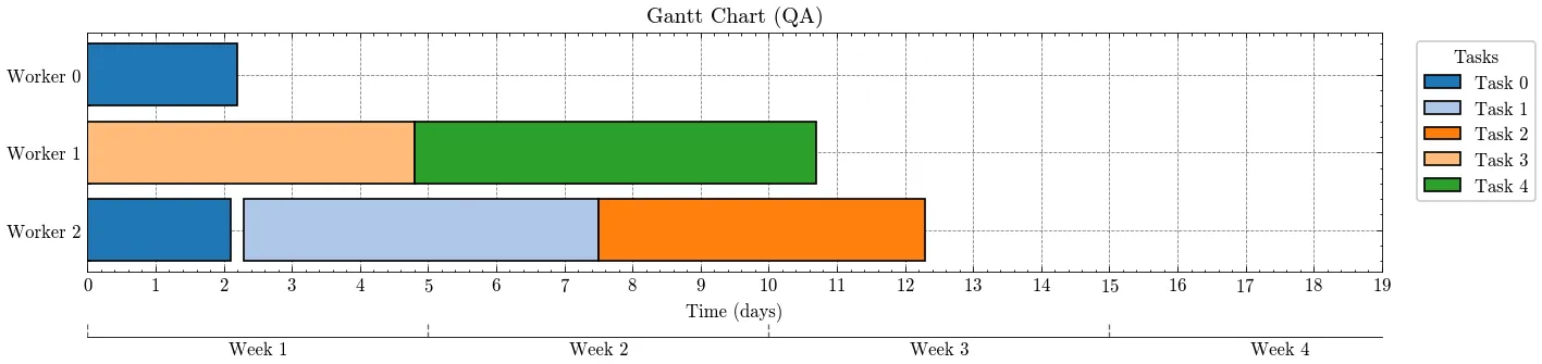
As analyzing the results in Figure 1, we can see that the solver successfully minimized the makespan to approximately 12 days (Term 1 effect) although the limit was 19 days. The output also demonstrates that tasks were assigned in the correct sequences (0→1→2 and 3→4) (Term 6 effect) and no multitasking occurred, as shown by the lack of overlapping bars (Term 4 effect). Furthermore, we can see that Tasks 0 and 1 were completed within their respective one-week and two-week windows (Term 5 effect).

Figure 1: Gantt chart results via quantum annealing

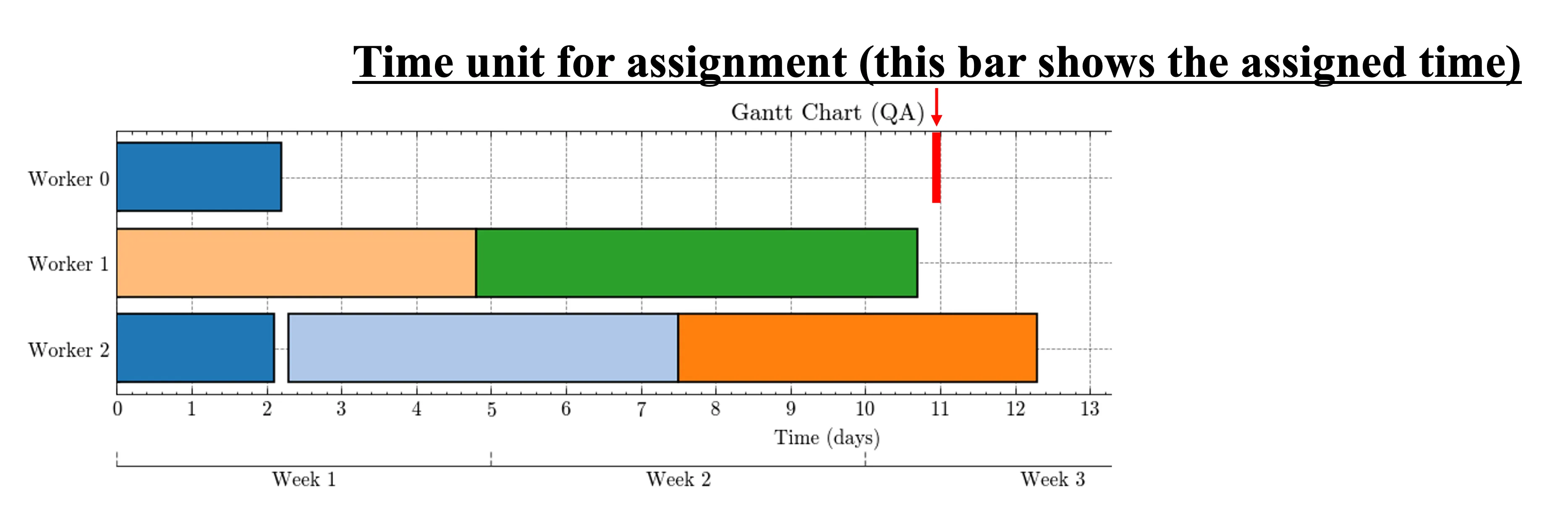
The red line in Figure 2 indicates the allocation at the smallest time unit. Notice that tasks are scheduled in continuous blocks rather than fragmented segments, ensuring high efficiency (Term 3 effect).

Figure 2: Minimum allocation unit on the Gantt chart

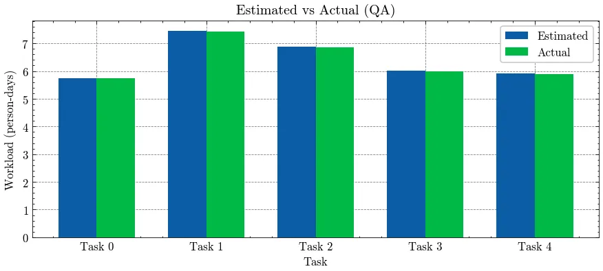
Finally, Figure 3 confirms that the actual assigned workload matches the required effort ($A_f$) for every task (Term 2 effect).

Figure 3: Comparison of assigned task volume and required task volume

These results prove that the QUBO formulation successfully produces a feasible and high-quality solution that is comparable to results from classical solvers like Gurobi.

---

4. Summary

This page provided a detailed explanation of the mathematical formulation for workforce scheduling and demonstrated how to achieve an optimized result by setting constant values. When formulating a problem in QUBO format, the most critical step is the mathematical representation of your specific requirements. Although the example used here is complex and advanced, it provides an excellent material to learn the essentials of optimization.

We encourage you to practice the translation of verbal requirements into mathematical equiations using simpler scheduling tasks or everyday examples. Building this intuition will eventually enables you to develop custom optimization models for a wide variety of real-world problems.

This research is currently being prepared for publication. Details are subject to change.

---

5. Writer

Second-year master’s student in the Ohzeki group at Graduate School of Information Sciences, Tohoku University

Kaito Yashiro

(Translated by Ami Koshikawa)